All of common grids were re-generated. The new file names were GridXM.grd. The reason why the common grids were changed is described in Comparison of original and modified common grids
The file names of all grids were modified from CaseX.grd to GridX.grd. However, the contents are not changed.
For investigation of grid dependence, 5 computational grids are prepared. You can use as many grids as you like.
In the following, grid information, namely topology, file format, dimensions, are described. In addition, you can download grid files at the bottom of this page.
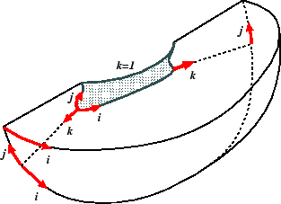
In Test Case 5, O-O type grid topology is used as shown in Fig.1. Types of boundary surfaces are summarized in Table 1.
| i=1 | y-symmetry plane before a ship |
| i=im | y-symmetry plane behind a ship |
| j=1 | y-symmetry plane under a ship |
| j=jm | z-symmetry plane |
| k=1 | ship surface |
| k=km | outer boundary |
The files to be downloaded are in ascii and plot3d format as follows:
      implicit real*8(x)

      write(20,*) nblk
      write(20,*) im,jm,km
      write(20,'(5g16.8)')
     $            (((x(1,i,j,k),i=1,im),j=1,jm),k=1,km),
     $            (((x(2,i,j,k),i=1,im),j=1,jm),k=1,km),
     $            (((x(3,i,j,k),i=1,im),j=1,jm),k=1,km)

        nblk	  : Number of grid. In this case, nblk=1.
        im,jm,km  : Number of grid points in xi, eta, zeta directions.
                      xi       circumferential direction
                      eta      girth(or depth) direction
                      zeta     normal direction
        x(m,i,j,k): Coordinates of grid points in right hand system
                      x(1,.. ) x-coordinate
                      x(2,...) y-coordinate
                      x(3,...) z-coordinate
The dimensions of 5 grids are summarized in Table 2. Grid3M.p3d was generated by deleting the alternate points along all grid lines of Grid1M.p3d as:
Similarily, Grid4M.p3d and Grid5M.p3d were also generated from Grid2M.p3d and Grid3M.p3d, respectively.
| grid name | im | jm | km | |
| Grid1M.p3d | 513 | 97 | 193 |
|
| Grid2M.p3d | 361 | 69 | 137 |
|
| Grid3M.p3d | 257 | 49 | 97 |
|
| Grid4M.p3d | 181 | 35 | 69 |
|
| Grid5M.p3d | 129 | 25 | 49 |
|
5 grid can be downloaded. All files are compressed in zip format.
Comparison of original and modified common grids