Complex Network Analysis of International Container Shipping Routes (2015.01.13)
DATA SYSTEM RESEARCH GROUP
Research Introduction of Data System Research Group
Complex Network Analysis of International Container Shipping Routes
We can represent shipping transportation activities as a network. For example, container ship voyages are schemed in advance, as shown in the callouts in Figure 1. For this data, if we represent ports as dots and ship movements between ports as lines, we can draw a network, as shown in the figure. (In networks, points are sometimes called nodes or vertices, and lines are called edges or links.) Here, we present a case study of an analysis of an international container shipping route network using methods from a relatively new field of research called complex networks.
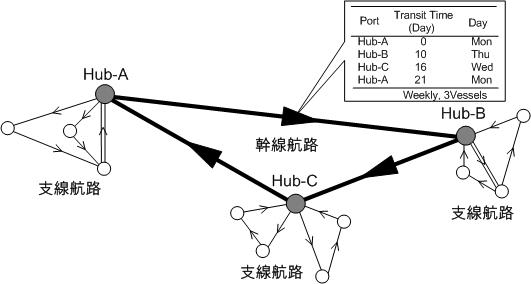
Figure 1 Network representation of container ship route data
Complex networks is a research field that has been developing in the wake of the two papers, with a series of reports on analyses of real networks in the real world and models that reproduce the properties of the analyzed networks. There are also a few reports on networks related to traffic and transportation that have been subject to analysis, although they are few. The networks representing complex networks are the small-world and scale-free networks shown below.
■Small-World Network(Watts, Strogatz, 1998(*1))
The Small World Network is proposed based on the hypothesis that the mechanism of synchronous phenomena (like the phenomenon of many fireflies flickering in synchrony) is related to its topology (the way nodes are connected). And the model that generates the small-world network is called the WS model, an acronym for the proposer. The Small World Network is known as the sixth order of separation. The network describes that anyone can reach each other by tracing six acquaintances. When you are talking with someone and find that you unexpectedly have an acquaintance in common, you may express that "the world is small," which is the very name for this phenomenon. For example, if you continue to pass strangers at an intersection: your friend, your friend's family member, your friend's family member's boss, and so on, it means that, on average, you will reach the person you just passed about six people ahead of you. This phenomenon is interesting because the number of intervening people is extremely minute relative to the world's population and is very out of tune with how people feel. Figure 2 shows a network consisting of a regularly connected network (left) and some (middle) or many (right) randomly reconnected links, which explains why phenomena such as sixth-order segues occur.
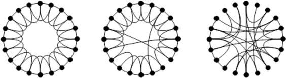
Figure 2 Illustration of the small world network
Before proceeding with the explanation, we present two indicators to capture the characteristics of this network. The first is the average distance between vertices, L, and the second is the clustering coefficient, C. Figure 3 is a network to illustrate this measure. (What we are concerned with here is how to connect the nodes via links, not the location of the nodes or the length or shape of the links.)
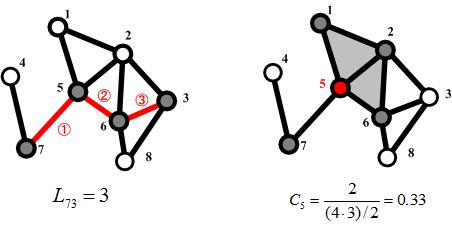
Figure 3 Illustration of indicators
The average distance between vertices is a measure like the 6 in "the 6th order of separation." The clustering coefficient, when applied to a network of friendships (we represent people by nodes and friendships by links), is a measure like the density of connections on a network because it is high when one's friends are friends mutually. (We know that you may realize that your topics are communicated easily to many people around you if you have a high clustering coefficient for yourself.)
Figure 4 shows the percentage of randomly reconnected links shown in Figure 2 as p on the horizontal axis. We can see that as p grows (as more links are bullshit-strung), both L and C decrease, but L decreases faster than C, and the state of being a large C and a small L remains over a wide range of p. This state is the mechanism that explains the phenomenon known as the sixth-order gap. Imagining the phenomenon of information transmission on a Small-World Network, we expect that information has the property of spreading quickly to all corners of the net. This situation is well-achieved through networks such as acquaintanceships, which is a network that is appreciated by those who are trying to promote some product because it makes it easier for that information to be all over. However, given the flu pandemic, it could be interpreted as an unfavorable network, as the virus could spread quickly over the Internet. Therefore, the judgment of good or bad depends on the network target.
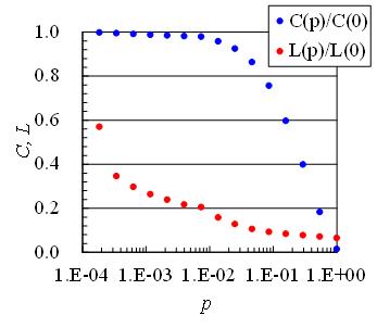
Figure 4 Relationship between the average distance between vertices L, clustering coefficient C, and the percentage p of links rearranged randomly.
■Scale-Free Network(Barabási, Albert 1999(*2))
The Scale-Free Network is discovered on the network formed by Internet homepages (through hyperlinks), and the model that generates the Scale-Free Network is called the BA model, an acronym for the proposer. The BA model generates a network that grows over time by a Preferential Attachment rule. The growth process is shown schematically in Figure 5. As time progresses, black nodes connect to white nodes connected to the network, but which white node they connect to is determined by a probability proportional to the degree of the white node. This fact means that nodes on a network with a large degree are more likely to be linked to newly added nodes. (In fact, if you set up a website on the Internet, you would expect to get more hits if you have a direct link to a well-known site than to an unknown site in the same field.)
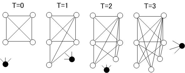
Figure 5 Schematic diagram of the preferential selection rule
Scale-free is the name of the lack of a representative scale, which implies a degree distribution. Figure 6 shows the order distribution of the 10000-node network generated by the BA model. This figure is drawn on a double-logarithmic graph with the order k on the horizontal axis and the frequency distribution (number of nodes) of nodes of that order on the vertical axis. In this figure, if there is a peak like a summit somewhere, it can be interpreted as a representative scale. But this figure shows a distribution with a declining right shoulder, and it is impossible to determine where the peak is. The straight line in the figure shows a line proportional to k-3, which is the theoretical analysis result of this model and is nearly identical to the slope of the plotted scatter plot.
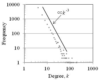
Figure 6 Order distribution of Scale-Free Network
We often give robustness as an example of a property of Scale-Free Networks. That is, the property that if we choose two nodes not removed at random, there is a high possibility that they are still connected on the network (there is a path connecting the two nodes) even if we destroy a portion of the network by removing a node. However, while this property appears when the selection of the removed nodes is bullshit, the network has the property that we can divide up easily when nodes with large orders, such as hub nodes, are selected for removal.
■International Container Shipping Route Network
Here, we will treat the service information (port call patterns) of international container ship routes shown in Figure 1 as a network and analyze it from the viewpoint of the complex network described so far. We used Container vessel schedule data for April 2010 provided by Containerisation International Online. Figure 1 schematically illustrates a container ship route. Container ship routes are similar to bus routes and railroads, with schedules published in advance. However, since most people who use trains and buses have a round-trip travel pattern, the movement of equipment for buses and trains is also almost in a round-trip pattern. Whereas for container ships, most movements are in circular patterns, visiting different ports on the outbound and inbound routes, as shown in Figure 1. This pattern is due to the distorted structure of the cargo: its movement is not back and forth like that of a person, and the demand is high in one direction. We also cite the containership network as a hub-and-spoke network. The hub-spoke network creates a great demand by aggregating smaller demand into a hub port through branch line routes. Big container vessels then transport great demand on long-haul trunk routes, reducing the cost per container. In other words, it is a transportation system that takes advantage of economies of scale by using large vessels for long-distance mass transportation. It is a universal transportation network found in cargo and human transportation systems and biological systems. All container ship routes in the data are drawn on a world map as links in a network, as shown in Figure 8. The inter-port links depicted in this figure are straight lines on the map, without regard to routes through the sea. We can see that so many shipping lanes stretch that continental coastlines remain hidden. When the number of links increases, as in Figure 8, we often grasp what is depicted with difficulty, even when drawing the network. In such cases, a technique called "edge bundling," as shown in Figure 7, may be used. This diagram is a technique to make it easier to see a network with many links by bundling links where the two nodes at either end are close to each other.
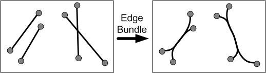
Figure 7 Image of edge bundle
Figure 9 uses edge bundles, and the greater the degree of overlap of the links, the more the white color is emphasized. Figure 9 with edge bundling shows the network structure more clearly than Figure 8, and the three major shipping routes, North America West Coast - Northeast Asia, Europe - North America East Coast, and Northeast Asia - Europe via Singapore, as well as regional networks within Asia, Europe, and the Caribbean, emerge as strong links connected by many links.
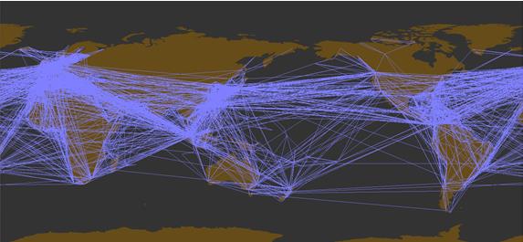
Figure 8 International container shipping route network (Links between all ports drawn as straight lines)
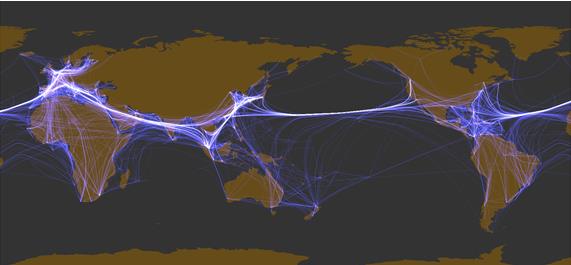
Figure 9 International container shipping route network (Processed by edge bundles)
The small-world, scale-free network analysis presented above for the international container shipping route network yields the results shown in Table 1 and Figure 10. In Table 1, N is the number of ports serving as nodes, M is the number of links, < k > is the average degree, L and C are the aforementioned average distance between vertices and clustering factor, and D, called the network diameter, means the largest Lij. The table also shows results for a random network of the same size (as shown on the right in Figure 2). From this, the network formed by container ship routes has an equivalent L and a larger C, compared with the random network, indicating its characteristics as a small-wart network. L=3.8 means that, on average, two ports are via 3.8 voyages, and D=15 shows that they are connected at most by 15 voyages. Figure 9 also shows the order distribution. The order distribution shows a linear decreasing trend on both logarithmic graphs, which seems near to a power distribution in a scale-free network. But the slope appears to be slightly different around the order 10 level. Although we must analyze the meaning of the emergence of different inclinations further, it is possible that the characteristics of the shipping network, which cannot pass through continents, may have an impact.
Table 1 Comparison of international container shipping route networks and random networks
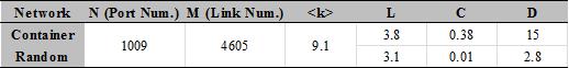
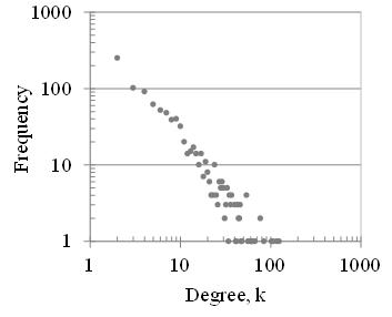
Figure 10 Order distribution of container shipping route network
These results indicate that the network formed by international container shipping routes has great potential to have the characteristics of a small-world, scale-free network. While the functional capability to transport containers everywhere with fewer voyages, the dysfunctional nature of a hub port can lead to significant disruptions at the level of network fragmentation.
*1 D.J. Watts and S.H. Strogatz, Collective dynamics of 'small-world' networks, Nature, Vol.393, pp.440-442, (1998)
*2 A.-L. Barabási and R. Albert, Emergence of scaling in random networks, Science, Vol.286, pp.509-512, (1999)